
קובץ:Window function and frequency response - Rectangular.svg

גודל התצוגה המקדימה הזאת מסוג PNG של קובץ ה־SVG הזה: 512 × 256 פיקסלים. רזולוציות אחרות: 320 × 160 פיקסלים | 640 × 320 פיקסלים | 1,024 × 512 פיקסלים | 1,280 × 640 פיקסלים | 2,560 × 1,280 פיקסלים.
לקובץ המקורי (קובץ SVG, הגודל המקורי: 512 × 256 פיקסלים, גודל הקובץ: 157 ק"ב)
| זהו קובץ שמקורו במיזם ויקישיתוף. תיאורו בדף תיאור הקובץ המקורי (בעברית) מוצג למטה. |
תקציר
| תיאור |
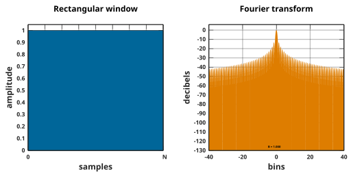
English: Window function and its Fourier transform: Rectangular window |
|||
| תאריך יצירה | ||||
| מקור | נוצר על־ידי מעלה היצירה | |||
| יוצר | Bob K (original version), Olli Niemitalo, BobQQ | |||
| אישורים והיתרים (שימוש חוזר בקובץ זה) |
אני, בעל זכויות היוצרים על עבודה זו, מפרסם בזאת את העבודה תחת הרישיון הבא:
|
|||
| גרסאות אחרות |
The SVG images generated by the enclosed Octave source code replace the older PNG images. See Window function (rectangular).png for example of writing .png files |
|||
| SVGהתפתחות | ||||
| Outputs | The script below generates these SVG images:
This Octave script is not MATLAB-compatible. Things you may need to install to run the script:
For viewing the svg files using "display", you may want to install:
|
|||
| Gnu Octave and Perl Scripts | Octave codegraphics_toolkit gnuplot
pkg load signal
% Characteristics common to both plots
set(0, "DefaultAxesFontName", "Microsoft Sans Serif")
set(0, "DefaultTextFontName", "Microsoft Sans Serif")
set(0, "DefaultAxesTitleFontWeight", "bold")
set(0, "DefaultAxesFontWeight", "bold")
set(0, "DefaultAxesFontSize", 20)
set(0, "DefaultAxesLineWidth", 3)
set(0, "DefaultAxesBox", "on")
set(0, "DefaultAxesGridLineStyle", "-")
set(0, "DefaultAxesGridColor", [0 0 0]) % black
set(0, "DefaultAxesGridAlpha", 0.25) % opaqueness of grid
set(0, "DefaultAxesLayer", "bottom") % grid not visible where overlapped by graph
%========================================================================
function plotWindow (w, wname, wfilename = "", wspecifier = "", wfilespecifier = "")
close % If there is a previous screen image, remove it.
M = 32; % Fourier transform size as multiple of window length
Q = 512; % Number of samples in time domain plot
P = 40; % Maximum bin index drawn
dr = 130; % (dynamic range) Maximum attenuation (dB) drawn in frequency domain plot
L = length(w);
B = L*sum(w.^2)/sum(w)^2; % noise bandwidth (bins)
n = [0 : 1/Q : 1];
w2 = interp1 ([0 : 1/(L-1) : 1], w, n);
if (M/L < Q)
Q = M/L;
endif
figure("position", [1 1 1200 600]) % width = 2×height, because there are 2 plots
% Plot the window function
subplot(1,2,1)
area(n,w2,"FaceColor", [0 0.4 0.6], "edgecolor", [0 0 0], "linewidth", 1)
g_x = [0 : 1/8 : 1]; % user defined grid X [start:spaces:end]
g_y = [0 : 0.1 : 1];
set(gca,"XTick", g_x)
set(gca,"YTick", g_y)
% Special y-scale if filename includes "flat top"
if(index(wname, "flat top"))
ylimits = [-0.1 1.05];
else
ylimits = [0 1.05];
endif
ylim(ylimits)
ylabel("amplitude","FontSize",28)
set(gca,"XTickLabel",[" 0"; " "; " "; " "; " "; " "; " "; " "; " N"])
grid("on")
xlabel("samples","FontSize",28)
#{
% This is a disabled work-around for an Octave bug, if you don't want to run the perl post-processor.
text(-.18, .4,"amplitude","rotation",90, "Fontsize", 28);
text(1.15, .4,"decibels", "rotation",90, "Fontsize", 28);
#}
%Construct a title from input arguments.
%The default interpreter is "tex", which can render subscripts and the following Greek character codes:
% \alpha \beta \gamma \delta \epsilon \zeta \eta \theta \vartheta \iota \kappa \lambda \mu \nu \xi \o
% \pi \varpi \rho \sigma \varsigma \tau \upsilon \phi \chi \psi \omega.
%
if (strcmp (wspecifier, ""))
title(cstrcat(wname," window"), "FontSize", 28)
elseif (length(strfind (wspecifier, "&#")) == 0 )
title(cstrcat(wname,' window (', wspecifier, ')'), "FontSize", 28)
else
% The specifiers '\sigma_t' and '\mu' work correctly in the output file, but not in subsequent thumbnails.
% So UNICODE substitutes are used. The tex interpreter would remove the & character, needed by the Perl script.
title(cstrcat(wname,' window (', wspecifier, ')'), "interpreter", "none", "FontSize", 28)
endif
ax1 = gca;
% Compute spectal leakage distribution
H = abs(fft([w zeros(1,(M-1)*L)]));
H = fftshift(H);
H = H/max(H);
H = 20*log10(H);
H = max(-dr,H);
n = ([1:M*L]-1-M*L/2)/M;
k2 = [-P : 1/M : P];
H2 = interp1 (n, H, k2);
% Plot the leakage distribution
subplot(1,2,2)
h = stem(k2,H2,"-");
set(h,"BaseValue",-dr)
xlim([-P P])
ylim([-dr 6])
set(gca,"YTick", [0 : -10 : -dr])
set(findobj("Type","line"), "Marker", "none", "Color", [0.8710 0.49 0])
grid("on")
set(findobj("Type","gridline"), "Color", [.871 .49 0])
ylabel("decibels","FontSize",28)
xlabel("bins","FontSize",28)
title("Fourier transform","FontSize",28)
text(-5, -126, ['B = ' num2str(B,'%5.3f')],"FontWeight","bold","FontSize",14)
ax2 = gca;
% Configure the plots so that they look right after the Perl post-processor.
% These are empirical values (trial & error).
% Note: Would move labels and title closer to axes, if I could figure out how to do it.
x1 = .08; % left margin for y-axis labels
x2 = .02; % right margin
y1 = .14; % bottom margin for x-axis labels
y2 = .14; % top margin for title
ws = .13; % whitespace between plots
width = (1-x1-x2-ws)/2;
height = 1-y1-y2;
set(ax1,"Position", [x1 y1 width height]) % [left bottom width height]
set(ax2,"Position", [1-width-x2 y1 width height])
%Construct a filename from input arguments.
if (strcmp (wfilename, ""))
wfilename = wname;
endif
if (strcmp (wfilespecifier, ""))
wfilespecifier = wspecifier;
endif
if (strcmp (wfilespecifier, ""))
savetoname = cstrcat("Window function and frequency response - ", wfilename, ".svg");
else
savetoname = cstrcat("Window function and frequency response - ", wfilename, " (", wfilespecifier, ").svg");
endif
print(savetoname, "-dsvg", "-S1200,600")
% close % Relocated to the top of the function
endfunction
%========================================================================
global N L
% Generate odd-length, symmetric windows
N = 2^16; % Large value ensures most accurate value of B
n = 0:N;
L = length(n); % Window length
%========================================================================
w = ones(1,L);
plotWindow(w, "Rectangular")
%========================================================================
w = 1 - abs(n-N/2)/(L/2);
plotWindow(w, "Triangular")
% Indistinguishable from Triangular for large N
% w = 1 - abs(n-N/2)/(N/2);
% plotWindow(w, "Bartlett")
%========================================================================
w = parzenwin(L).';
plotWindow(w, "Parzen");
%========================================================================
w = 1-((n-N/2)/(N/2)).^2;
plotWindow(w, "Welch");
%========================================================================
w = sin(pi*n/N);
plotWindow(w, "Sine")
%========================================================================
w = 0.5 - 0.5*cos(2*pi*n/N);
plotWindow(w, "Hann")
%========================================================================
w = 0.53836 - 0.46164*cos(2*pi*n/N);
plotWindow(w, "Hamming", "Hamming", 'a_0 = 0.53836', "alpha = 0.53836")
%========================================================================
w = 0.42 - 0.5*cos(2*pi*n/N) + 0.08*cos(4*pi*n/N);
plotWindow(w, "Blackman")
%========================================================================
w = 0.355768 - 0.487396*cos(2*pi*n/N) + 0.144232*cos(4*pi*n/N) -0.012604*cos(6*pi*n/N);
plotWindow(w, "Nuttall", "Nuttall", "continuous first derivative")
%========================================================================
w = 0.3635819 - 0.4891775*cos(2*pi*n/N) + 0.1365995*cos(4*pi*n/N) -0.0106411*cos(6*pi*n/N);
plotWindow(w, "Blackman-Nuttall", "Blackman-Nuttall")
%========================================================================
w = 0.35875 - 0.48829*cos(2*pi*n/N) + 0.14128*cos(4*pi*n/N) -0.01168*cos(6*pi*n/N);
plotWindow(w, "Blackman-Harris", "Blackman-Harris")
%========================================================================
% Matlab coefficients
a = [0.21557895 0.41663158 0.277263158 0.083578947 0.006947368];
% Stanford Research Systems (SRS) coefficients
% a = [1 1.93 1.29 0.388 0.028];
% a = a / sum(a);
w = a(1) - a(2)*cos(2*pi*n/N) + a(3)*cos(4*pi*n/N) -a(4)*cos(6*pi*n/N) +a(5)*cos(8*pi*n/N);
plotWindow(w, "flat top")
%========================================================================
% The version using \sigma no longer renders correct thumbnail previews.
% Ollie's older version using σ seems to solve that problem.
sigma = 0.4;
w = exp(-0.5*( (n-N/2)/(sigma*N/2) ).^2);
% plotWindow(w, "Gaussian", "Gaussian", '\sigma = 0.4', "sigma = 0.4")
plotWindow(w, "Gaussian", "Gaussian", "σ = 0.4", "sigma = 0.4")
%========================================================================
% Confined Gaussian
global T P abar target_stnorm
N = 512; % Reduce N to avoid excessive computation time
n = 0:N;
L = length(n); % Window length
target_stnorm = 0.1;
function [g,sigma_w,sigma_t] = CGWn(alpha, M)
% determine eigenvectors of M(alpha)
global L P T
opts.maxit = 10000;
if(M ~= L)
[g,lambda] = eigs(P + alpha*T, M, 'sa', opts);
else
[g,lambda] = eig(P + alpha*T);
end
sigma_t = sqrt(diag((g'*T*g) / (g'*g)));
sigma_w = sqrt(diag((g'*P*g) / (g'*g)));
end
function [h1] = helperCGW(anorm)
global L abar target_stnorm
[~,~,sigma_t] = CGWn(anorm*abar,1);
h1 = sigma_t - target_stnorm * L;
end
% define alphabar, and matrices T and P
T = zeros(L,L);
P = zeros(L,L);
for m=1:L
T(m,m) = (m - (L+1)/2)^2;
for l=1:L
if m ~= l
P(m,l) = 2*(-1)^(m-l)/(m-l)^2;
else
P(m,l) = pi^2/3;
end
end
end
abar = (10/L)^4/4;
[anorm, aval] = fzero(@helperCGW, 0.1/target_stnorm);
[CGWg, CGWsigma_w, CGWsigma_t] = CGWn(anorm*abar,1);
sigma_t = CGWsigma_t/L % Confirm sigma_t
w = CGWg * sign(mean(CGWg));
w = w'/max(w);
% \sigma_t works correctly in actual file, but not in thumbnail versions.
% plotWindow(w, "Confined Gaussian", "Confined Gaussian", '\sigma_t = 0.1', "sigma_t = 0.1");
plotWindow(w, "Confined Gaussian", "Confined Gaussian", "σₜ = 0.1", "sigma_t = 0.1");
N = 2^16; % restore original N
n = 0:N;
L = length(n); % Window length
%========================================================================
global denominator;
sigma = 0.1;
denominator = (2*L*sigma).^2;
function [gaussout] = gauss(x)
global N denominator
gaussout = exp(- (x-N/2).^2 ./ denominator);
end
w = gauss(n) - gauss(-1/2).*(gauss(n+L) + gauss(n-L))./(gauss(-1/2 + L) + gauss(-1/2 - L));
% \sigma_t works correctly in actual file, but not in thumbnail versions
% plotWindow(w, "App. conf. Gaussian", "Approximate confined Gaussian", '\sigma_t = 0.1', "sigma_t = 0.1");
plotWindow(w, "App. conf. Gaussian", "Approximate confined Gaussian", "σₜ = 0.1", "sigma_t = 0.1");
%========================================================================
alpha = 0.5;
a = alpha*N/2;
w = ones(1,L);
m = 0 : a;
if( max(m) == a )
m = m(1:end-1);
endif
M = length(m);
w(1:M) = 0.5*(1-cos(pi*m/a));
w(L:-1:L-M+1) = w(1:M);
% plotWindow(w, "Tukey", "Tukey", '\alpha = 0.5', "alpha = 0.5")
plotWindow(w, "Tukey", "Tukey", "α = 0.5", "alpha = 0.5")
%========================================================================
epsilon = 0.1;
a = N*epsilon;
w = ones(1,L);
m = 0 : a;
if( max(m) == a )
m = m(1:end-1);
endif
% Divide by 0 is handled by Octave. Results in w(1) = 0.
z_exp = a./m - a./(a-m);
M = length(m);
w(1:M) = 1 ./ (exp(z_exp) + 1);
w(L:-1:L-M+1) = w(1:M);
#{
% The original method is harder to understand:
t_cut = N/2 - a;
T_in = abs(n - N/2);
z_exp = (t_cut - N/2) ./ (T_in - t_cut)...
+ (t_cut - N/2) ./ (T_in - N/2);
% The numerator forces sigma = 0 at n = 0:
sigma = (T_in < N/2) ./ (exp(z_exp) + 1);
% Either the 1st term or the 2nd term is 0, depending on n:
w = 1 * (T_in <= t_cut) + sigma .* (T_in > t_cut);
#}
% plotWindow(w, "Planck-taper", "Planck-taper", '\epsilon = 0.1', "epsilon = 0.1")
plotWindow(w, "Planck-taper", "Planck-taper", "ε = 0.1", "epsilon = 0.1")
%========================================================================
N = 2^12; % Reduce N to avoid excess memory requirement
n = 0:N;
L = length(n); % Window length
alpha = 2;
s = sin(alpha*2*pi/L*[1:N])./[1:N];
c0 = [alpha*2*pi/L,s];
A = toeplitz(c0);
[V,evals] = eigs(A, 1);
[emax,imax] = max(abs(diag(evals)));
w = abs(V(:,imax));
w = w.';
w = w / max(w);
% plotWindow(w, "DPSS", "DPSS", '\alpha = 2', "alpha = 2")
plotWindow(w, "DPSS", "DPSS", "α = 2", "alpha = 2")
%========================================================================
alpha = 3;
s = sin(alpha*2*pi/L*[1:N])./[1:N];
c0 = [alpha*2*pi/L,s];
A = toeplitz(c0);
[V,evals] = eigs(A, 1);
[emax,imax] = max(abs(diag(evals)));
w = abs(V(:,imax));
w = w.';
w = w / max(w);
% plotWindow(w, "DPSS", "DPSS", '\alpha = 3', "alpha = 3")
plotWindow(w, "DPSS", "DPSS", "α = 3", "alpha = 3")
N = 2^16; % Restore original N
n = 0:N;
L = length(n); % Window length
%========================================================================
alpha = 2;
w = besseli(0,pi*alpha*sqrt(1-(2*n/N -1).^2))/besseli(0,pi*alpha);
% plotWindow(w, "Kaiser", "Kaiser", '\alpha = 2', "alpha = 2")
plotWindow(w, "Kaiser", "Kaiser", "α = 2", "alpha = 2")
%========================================================================
alpha = 3;
w = besseli(0,pi*alpha*sqrt(1-(2*n/N -1).^2))/besseli(0,pi*alpha);
% plotWindow(w, "Kaiser", "Kaiser", '\alpha = 3', "alpha = 3")
plotWindow(w, "Kaiser", "Kaiser", "α = 3", "alpha = 3")
%========================================================================
alpha = 5; % Attenuation in 20 dB units
w = chebwin(L, alpha * 20).';
% plotWindow(w, "Dolph-Chebyshev", "Dolph-Chebyshev", '\alpha = 5', "alpha = 5")
plotWindow(w, "Dolph–Chebyshev", "Dolph-Chebyshev", "α = 5", "alpha = 5")
%========================================================================
w = ultrwin(L, -.5, 100, 'a')';
% \mu works correctly in actual file, but not in thumbnail versions
% plotWindow(w, "Ultraspherical", "Ultraspherical", '\mu = -0.5', "mu = -0.5")
plotWindow(w, "Ultraspherical", "Ultraspherical", "μ = -0.5", "mu = -0.5")
%========================================================================
tau = (L/2);
w = exp(-abs(n-N/2)/tau);
% plotWindow(w, "Exponential", "Exponential", '\tau = N/2', "half window decay")
plotWindow(w, "Exponential", "Exponential", "τ = N/2", "half window decay")
%========================================================================
tau = (L/2)/(60/8.69);
w = exp(-abs(n-N/2)/tau);
% plotWindow(w, "Exponential", "Exponential", '\tau = (N/2)/(60/8.69)', "60dB decay")
plotWindow(w, "Exponential", "Exponential", "τ = (N/2)/(60/8.69)", "60dB decay")
%========================================================================
w = 0.62 -0.48*abs(n/N -0.5) -0.38*cos(2*pi*n/N);
plotWindow(w, "Bartlett-Hann", "Bartlett-Hann")
%========================================================================
alpha = 4.45;
epsilon = 0.1;
t_cut = N * (0.5 - epsilon);
t_in = n - N/2;
T_in = abs(t_in);
z_exp = ((t_cut - N/2) ./ (T_in - t_cut) + (t_cut - N/2) ./ (T_in - N/2));
sigma = (T_in < N/2) ./ (exp(z_exp) + 1);
w = (1 * (T_in <= t_cut) + sigma .* (T_in > t_cut)) .* besseli(0, pi*alpha * sqrt(1 - (2 * t_in / N).^2)) / besseli(0, pi*alpha);
% plotWindow(w, "Planck-Bessel", "Planck-Bessel", '\epsilon = 0.1, \alpha = 4.45', "epsilon = 0.1, alpha = 4.45")
plotWindow(w, "Planck–Bessel", "Planck-Bessel", "ε = 0.1, α = 4.45", "epsilon = 0.1, alpha = 4.45")
%========================================================================
alpha = 2;
w = 0.5*(1 - cos(2*pi*n/N)).*exp( -alpha*abs(N-2*n)/N );
% plotWindow(w, "Hann-Poisson", "Hann-Poisson", '\alpha = 2', "alpha = 2")
plotWindow(w, "Hann–Poisson", "Hann-Poisson", "α = 2", "alpha = 2")
%========================================================================
w = sinc(2*n/N - 1);
plotWindow(w, "Lanczos")
%========================================================================
% optimized Nutall
ak = [-1.9501232504232442 1.7516390954528638 -0.9651321809782892 0.3629219021312954 -0.0943163918335154 ...
0.0140434805881681 0.0006383045745587 -0.0009075461792061 0.0002000671118688 -0.0000161042445001];
n = -N/2:N/2;
n = n/std(n);
w = 1;
for k = 1 : length(ak)
% This is an array addition, which expands the dimension of w[] as needed, and the value "1" is replicated.
w = w + ak(k)*(n.^(2*k));
endfor
w = w/max(w);
plotWindow(w, "GAP optimized Nuttall")
Perl code#!/usr/bin/perl
opendir (DIR, '.') or die $!; ## open the current directory , if error exit
while ($file = readdir(DIR)) { ## read all the file names in the current directory
$ext = substr($file, length($file)-4); ## get the last 4 letters of the file name
if ($ext eq '.svg') { ## if the file extension is '.svg'
print("$file\n"); ## print file name
($pre, $name) = split(" - ", substr($file, 0, length($file)-4)); ## split the filename in 2
@lines = (); ## dummy up an array
open (INPUTFILE, "<", $file) or die $!; ## open up the file for reading
while ($line = <INPUTFILE>) { ## loop through all the lines in the file
$line =~ s/&/&/g; ## replace "&" with "&" , get rid of semicolon
if ($line eq "<title>Gnuplot</title>\n") { ## if line is EXACTLY equal to "<.....>\n" then
$line = '<title>Window function and its Fourier transform – '.$name."</title>"."\n"; ## set the line to a new value, – - is unicode for a dash
## the .$name. concatenates the strings together
} ## end if
@lines[0+@lines] = $line; ## append to the output array the value of the modified line
} ## end loop
close(INPUTFILE); ## close the input file
open (OUTPUTFILE, ">", $file) or die $!; ## open the output file
for ($t = 0; $t < @lines; $t++) { ## loop through the output array, printing out each line
print(OUTPUTFILE $lines[$t]);
} ## end loop
close(OUTPUTFILE); ## close the output file
} ## end if
} ## end loop
closedir (DIR); ## close the directory
|
.png)
.png#Octave_commands)
.svg)
.svg)
.svg)
.svg)
.svg)
.svg)
.svg)
.svg)
.svg)
.svg)
.svg)
.svg)
.svg)
.svg)
.svg)
.svg)
.svg)
.svg)
.svg)
.svg)
היסטוריית הקובץ
ניתן ללחוץ על תאריך/שעה כדי לראות את הקובץ כפי שנראה באותו זמן.
| תאריך/שעה | תמונה ממוזערת | ממדים | משתמש | הערה | |
|---|---|---|---|---|---|
| נוכחית | 20:48, 20 בנובמבר 2019 | | 256 × 512 (157 ק"ב) | Bob K | Display parameter B on frequency distribution |
| 01:54, 6 באפריל 2019 |  | 256 × 512 (156 ק"ב) | Bob K | Change xticks label from N-1 to N, because of changes to article [Window function] | |
| 23:27, 16 בפברואר 2013 |  | 256 × 512 (131 ק"ב) | Olli Niemitalo | Frequency response --> Fourier transform | |
| 12:18, 13 בפברואר 2013 |  | 256 × 512 (131 ק"ב) | Olli Niemitalo | Font, dB range | |
| 06:01, 13 בפברואר 2013 |  | 256 × 512 (131 ק"ב) | Olli Niemitalo | User created page with UploadWizard |
שימוש בקובץ
![]() אין בוויקיפדיה דפים המשתמשים בקובץ זה.
אין בוויקיפדיה דפים המשתמשים בקובץ זה.
שימוש גלובלי בקובץ
אתרי הוויקי השונים הבאים משתמשים בקובץ זה:
- שימוש באתר en.wikipedia.org
- שימוש באתר pl.wikipedia.org