
קובץ:Solar AM0 spectrum with visible spectrum background (no).png

גודל התצוגה המקדימה הזאת: 800 × 494 פיקסלים. רזולוציות אחרות: 320 × 198 פיקסלים | 640 × 395 פיקסלים | 1,024 × 632 פיקסלים | 1,280 × 790 פיקסלים | 1,882 × 1,162 פיקסלים.
לקובץ המקורי (1,882 × 1,162 פיקסלים, גודל הקובץ: 182 ק"ב, סוג MIME: image/png)
| זהו קובץ שמקורו במיזם ויקישיתוף. תיאורו בדף תיאור הקובץ המקורי (בעברית) מוצג למטה. |
.png)
.png?uselang=he)
תקציר
| תיאור |
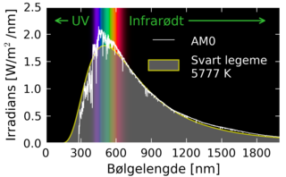
English: Solar AM0 (Air Mass Zero) spectrum (Chris A. Gueymard 2002) as included in SMARTS 2.95, together with a blackbody spectrum for 5777 kelvin and solid angle 2.16e-5*π steradian for the source (the solar disk). The visible region of the electromagnetic spectrum is shown using the CIE visible spectrum as implemented in ColorPy by Mark Kness (2008). Figure with Norwegian Bokmål labels. |
| תאריך יצירה | |
| מקור | נוצר על־ידי מעלה היצירה, created using Matplotlib |
| יוצר | Danmichaelo |
| גרסאות אחרות | Version with English labels |
.png)
| Source |
|---|
#encoding=utf8

import matplotlib
from matplotlib import rc
from matplotlib import pyplot as plt
import numpy as np

rc('lines', linewidth=0.5)
rc('font', family='sans-serif', size=10)
rc('axes', labelsize=10)
rc('xtick', labelsize=9)
rc('ytick', labelsize=9)

golden_mean = (np.sqrt(5)-1.0)/2.0
inches_per_cm = 1.0/2.54
fig_width = 8 * inches_per_cm
fig_height = golden_mean * fig_width
fig = plt.figure(figsize = [fig_width, fig_height])

from colorpy import ciexyz, colormodels

Fs = 2.16e-5 * np.pi;   # Geometrical factor of sun as viewed from Earth
h = 6.63e-34;           # Boltzmann const. [Js]
c = 3.e8;               # speed of light [m/s]
q = 1.602e-19;          # electron charge [C]

def blackbody(wvlgth, temp):
    # per nanometer 1e-9:
    fac = (2 * Fs * h * c**2) / ((wvlgth * 1.e-9)**5)
    return fac / (np.exp(1240./(wvlgth*8.62e-5*temp)) - 1) * 1.e-9

def draw_vis_spec(ax, ymax):
    spectrum = ciexyz.empty_spectrum()[:,0]
    (num_wl,) = spectrum.shape
    rgb_colors = np.empty((num_wl, 3))
    for i in xrange (0, num_wl):
        xyz = ciexyz.xyz_from_wavelength(spectrum[i])
        rgb = colormodels.rgb_from_xyz(xyz)
        rgb_colors [i] = rgb
    rgb_colors /= np.max(rgb_colors) # scale to make brightest rgb value = 1.0

    num_points = len(spectrum)
    for i in xrange (0, num_points-1):
        x0 = spectrum[i]
        x1 = spectrum[i+1]
        y0 = 0.0
        y1 = ymax
        poly_x = [x0, x1, x1, x0]
        poly_y = [y0, y0, y1, y1]
        color_string = colormodels.irgb_string_from_rgb(rgb_colors [i])
        ax.fill(poly_x, poly_y, color_string, edgecolor=color_string)

ax = fig.add_subplot(111)

frame = ax.get_frame()
frame.set_facecolor('black')
xmax = 2000
ymax = 2.5

# Visible spectrum:

draw_vis_spec(ax, ymax)

# Blackbody:

temp = 5777
x = np.arange(100, 2000)
y = blackbody(x, temp)
y[-1] = 0.
ax.fill(x, y, '0.5', alpha = 0.7, linewidth = 0.9, edgecolor='yellow', label = 'Svart legeme\n%d K' % temp)

# AM0 spectrum:

d = np.loadtxt('smarts295.ext.txt', skiprows = 1)
x = d[:,0]
y = d[:,1]
y[0] = 0.
y[-1] = 0.
ax.plot(x, y, color='white', linewidth=0.5, label = 'AM0')
ax.set_xlim(0, xmax)
ax.set_xticks(np.arange(0, 1999, 300))
ax.set_ylim(0, ymax)

# Tweak, tweak and annotate:

texty = 2.25
ax.annotate('UV', xy = (50,texty), xytext = (230,texty), xycoords = 'data',
        horizontalalignment='left', verticalalignment='center', color='#33bb33',
        arrowprops = dict(arrowstyle='->', color='#33bb33'))
#ax.annotate('Synlig', xy=(400,texty), xycoords='data',
#        horizontalalignment='left', verticalalignment='center', color='white')
ax.annotate(u'Infrarødt', xytext = (720,texty), xy = (1900,texty), xycoords = 'data',
        horizontalalignment='left', verticalalignment='center', color='#33bb33',
        arrowprops = dict(arrowstyle='->',color='#33bb33'))

leg = ax.legend(loc='upper right', frameon=False, bbox_to_anchor = (1.0, 0.90) )
txts = leg.get_texts()
for txt in txts:
    txt.set_color('white')
    txt.set_fontsize(9)

ax.tick_params(color='white', labelcolor='black')
for spine in ax.spines.values():
    spine.set_edgecolor('white')
    spine.set_linewidth(1.4)

fig.subplots_adjust(left=0.16, bottom = 0.19, right=0.98, top=0.96)

ax.set_xlabel(u'Bølgelengde [nm]')
ax.set_ylabel(u'Irradians [W/m$^2$/nm]')
fig.savefig('Solar AM0 spectrum with visible spectrum background (no).png',dpi=600)
|
רישיון
| ברצוני, בעלי זכויות היוצרים על יצירה זו, לשחרר יצירה זו לנחלת הכלל. זה תקף בכל העולם. יש מדינות שבהן הדבר אינו אפשרי על פי חוק, אם כך: אני מעניק לכל אחד את הזכות להשתמש בעבודה זו לכל מטרה שהיא, ללא תנאים כלשהם, אלא אם כן תנאים כאלה נדרשים על פי חוק. |
היסטוריית הקובץ
ניתן ללחוץ על תאריך/שעה כדי לראות את הקובץ כפי שנראה באותו זמן.
| תאריך/שעה | תמונה ממוזערת | ממדים | משתמש | הערה | |
|---|---|---|---|---|---|
| נוכחית | 23:16, 16 במאי 2012 | | 1,162 × 1,882 (182 ק"ב) | Danmichaelo | slightly thicker line |
| 22:30, 16 במאי 2012 |  | 1,162 × 1,882 (181 ק"ב) | Danmichaelo | tweaks to make the figure more readable | |
| 22:12, 16 במאי 2012 |  | 1,162 × 1,882 (171 ק"ב) | Danmichaelo |
שימוש בקובץ
![]() אין בוויקיפדיה דפים המשתמשים בקובץ זה.
אין בוויקיפדיה דפים המשתמשים בקובץ זה.
.png)