
קובץ:Savitzky-golay pic gaussien bruite.svg

גודל התצוגה המקדימה הזאת מסוג PNG של קובץ ה־SVG הזה: 610 × 407 פיקסלים. רזולוציות אחרות: 320 × 214 פיקסלים | 640 × 427 פיקסלים | 1,024 × 683 פיקסלים | 1,280 × 854 פיקסלים | 2,560 × 1,708 פיקסלים.
לקובץ המקורי (קובץ SVG, הגודל המקורי: 610 × 407 פיקסלים, גודל הקובץ: 43 ק"ב)
| זהו קובץ שמקורו במיזם ויקישיתוף. תיאורו בדף תיאור הקובץ המקורי (בעברית) מוצג למטה. |
תקציר
| תיאור |
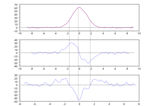
English: Savitzky-Golay algorithm (3rd degree polynomial, 9 points) applied on a gaussian peak with random noise: smoothing (top), first derivation (middle), second derivation (bottom).
The dashed lines highlight the zeros of the second dérivative (inflection points of the peak) and its minimum (top of the peak). Created with Scilab, processed with Inkscape.Français : Application de l'algorithme de Savitzky-Golay sur un pic gaussien bruité (polynôme de degré 3, 9 points) : lissage (haut), dérivée (milieu), dérivée seconde (bas).
Les traits pointillés mettent en évidence l'annulation de la dérivée seconde (points d'inflexion du pic) et son minimum (sommet du pic). Créé avec Scilab, retravaillé avec Inkscape. |
| תאריך יצירה | |
| מקור | נוצר על־ידי מעלה היצירה |
| יוצר | Christophe Dang Ngoc Chan |
| SVGהתפתחות |  English: English version by default.
Français : Version française, si les préférences de votre compte sont réglées (voir Special:Preferences). Scilab עם נוצרה ה גרפיקה וקטורית This file uses embedded text. |
| קוד מקור | (1) File generateur_pic_bruit.sce : generates a set of data and save it in the file noisy_gaussian_peak.txt.
SciLab code// **********
// Constants and initialisation
// **********
clear;
chdir("mypath/");
// parameters of the noisy curve
paramgauss(1) = 60; // height of the gaussian curve
paramgauss(2) = 3; // "width" of the gaussian curve
var=0.01; // variance of the noise normal law
nbpts = 100 // nombre of points
halfwidth = 3*paramgauss(2) // range for x
step = 2*halfwidth/nbpts;
// **********
// Fonctions
// **********
// gaussian peak
function [y] = gauss(A, x)
// A(1) : height of the peak
// A(2) : "width" of the peak
y = A(1)*exp(-x.^2/A(2));
endfunction
// **********
// Main program
// **********
// Generation of data
for i=1:nbpts
x = step*i - halfwidth;
X(i) = x;
Y(i) = gauss([paramgauss], x) + rand(var, "normal");
end
// Saving the data
write ("noisy_gaussian_peak.txt", [X, Y])
(2) File savitzkygolay.sce : processes the data.
Data// **********
// Constants and initialisation
// **********
clear;
clf;
chdir("mypath/")
// smoothing parameters :
width = 9; // width of the sliding window (number of pts)
poldeg = 3; // degree of the polynomial
// **********
// Functions
// **********
// Convolution coefficients
function [a]=convolcoefs(m, d)
// m : width of the window (number of pts)
// d : degree of the polynomial
l = (m-1)/2; // half-width of the window
z = (-l:l)'; // standardised abscissa
J = ones(m,d+1);
for i = 2:d+1
J(:,i) = z.^(i-1); // jacobian matrix
end
A = (J'*J)^(-1)*J';
a = A(1:3,:);
endfunction
// smoothing, determination of the first and second derivatives
function [y, yprime, ysecond] = savitzkygolay(X, Y, width, deg)
// X, Y: collection of data
// width: width of the window (number of pts)
// deg: degree of the polynomial
n = size(X, "*");
l = floor(width/2);
step = (X($)-X(1))/(n - 1);
y = Y;
yprime=zeros(Y);
ysecond=yprime;
a = convolcoefs(width, deg);
a(2,:) = 1/step*a(2,:);
a(3,:) = 2/step^2*a(2,:);
for i = 1:width
Ymat(i, :) = Y(i: n-width+i)';
end
solution = a*Ymat;
y = solution(1, :)';
yprime = solution(2, :)';
ysecond = solution(3, :)';
endfunction
// **********
// Main program
// **********
// data reading
data = read("noisy_gaussian_peak.txt", -1, 2)
Xinit = data(:,1);
Yinit = data(:,2);
//subplot(3,1,1)
//plot(Xdef, Ydef, "b")
// Data processing
[Ysmooth, Yprime, Ysecond] = savitzkygolay(Xinit, Yinit, width, poldeg);
// Display
offset = floor(width/2);
nbpts = size(Xinit, "*");
X1 = Xinit((offset+1):(nbpts-offset)); // removal of non-smotthed points
subplot(3,1,1)
plot(Xinit, Yinit, "b")
plot(X1, Ysmooth, "r")
subplot(3,1,2)
plot(X1, Yprime, "b")
subplot(3,1,3)
plot(X1, Ysecond, "b")
(3) When the sampling step is not constant, i.e. xi - xi - 1 varies, then it is possible to determine the polynomial by multi-linear regression. Text// **********
// Constants and initialisation
// **********
clear;
clf;
chdir("mypath\")
// smoothing parameters
width = 9; // width of the sliding window (number of pts)
// **********
// Functions
// **********
// 3rd degree polynomial
function [y]=poldegthree(A, x)
// Horner method
y = ((A(1).*x + A(2)).*x + A(3)).*x + A(4);
endfunction
// regression with the 3rd degree polynomial
function [A]=regression(X, Y)
// X, Y: column vectors of "width" values ;
// determines the polynomial of degree 3
// a*x^2 + b*x^2 + c*x + d
// by regression on (X, Y)
XX = [X.^3; X.^2; X];
[a, b, sigma] = reglin(XX, Y);
A = [a, b];
endfunction
// smoothing, determination of the first and second derivatives
function [y, yprime, ysecond] = savitzkygolay(X, Y, larg)
// X, Y: collection of data
n = size(X, "*");
l = floor(larg/2); // halfwidth
y=Y;
yprime=zeros(Y);
ysecond=yprime;
for i=(l+1):(n-l)
intervX = X((i-l):(i+l),1);
intervY = Y((i-l):(i+l),1);
Aopt = regression(intervX', intervY');
x = X(i);
y(i) = poldegthree(Aopt,x);
// Yfoo=poldegthree(Aopt,intervX);
// subplot(3,1,1) ; plot(intervX, Yfoo, "r")
yprime(i) = (3*Aopt(1)*x + 2*Aopt(2))*x + Aopt(3); // Horner
ysecond(i) = 6*Aopt(1)*x + 2*Aopt(2);
end
endfunction
// **********
// Main program
// **********
// data reading
data = read("noisy_gaussian_peak.txt", -1, 2)
Xinit = data(:,1);
Yinit = data(:,2);
//subplot(3,1,1)
//plot(Xdef, Ydef, "b")
// Data processing
[Ysmooth, Yprime, Ysecond] = savitzkygolay(Xinit, Yinit, width);
// Display
offset = floor(width/2);
nbpts = size(Xinit, "*");
vector1 = (offset+1):(nbpts-offset); // suppresion des points non-lissés
X1 = Xinit(vector1);
Y0 = Yliss(vector1)
Y1 = Yprime(vector1);
Y2 = Ysecond(vector1);
subplot(3,1,1)
plot(Xinit, Yinit, "b")
plot(X1, Y0, "r")
subplot(3,1,2)
plot(X1, Y1, "b")
subplot(3,1,3)
plot(X1, Y2, "b")
|
רישיון
אני, בעל זכויות היוצרים על היצירה הזאת, מפרסם אותה בזאת תחת הרישיונות הבאים:

|
מוענקת בכך הרשות להעתיק, להפיץ או לשנות את המסמך הזה, לפי תנאי הרישיון לשימוש חופשי במסמכים של גנו, גרסה 1.2 או כל גרסה מאוחרת יותר שתפורסם על־ידי המוסד לתוכנה חופשית; ללא פרקים קבועים, ללא טקסט עטיפה קדמית וללא טקסט עטיפה אחורית. עותק של הרישיון כלול בפרק שכותרתו הרישיון לשימוש חופשי במסמכים של גנו. |
הקובץ הזה מתפרסם לפי תנאי רישיונות קריאייטיב קומונז ייחוס-שיתוף זהה 3.0 לא מותאם, 2.5 כללי, 2.0 כללי ו־1.0 כללי.
- הנכם רשאים:
- לשתף – להעתיק, להפיץ ולהעביר את העבודה
- לערבב בין עבודות – להתאים את העבודה
- תחת התנאים הבאים:
- ייחוס – יש לתת ייחוס הולם, לתת קישור לרישיון, ולציין אם נעשו שינויים. אפשר לעשות את זה בכל צורה סבירה, אבל לא בשום צורה שמשתמע ממנה שמעניק הרישיון תומך בך או בשימוש שלך.
- שיתוף זהה – אם תיצרו רמיקס, תשנו, או תבנו על החומר, חובה עליכם להפיץ את התרומות שלך לפי תנאי רישיון זהה או תואם למקור.
הנכם מוזמנים לבחור את הרישיון הרצוי בעיניכם.
היסטוריית הקובץ
ניתן ללחוץ על תאריך/שעה כדי לראות את הקובץ כפי שנראה באותו זמן.
| תאריך/שעה | תמונה ממוזערת | ממדים | משתמש | הערה | |
|---|---|---|---|---|---|
| נוכחית | 16:07, 9 בנובמבר 2012 | | 407 × 610 (43 ק"ב) | Cdang | dashed line to highlight the inimum of the second derivative |
| 13:50, 9 בנובמבר 2012 |  | 407 × 610 (43 ק"ב) | Cdang | {{Information | description = {{en|1=Savitzky-Golay algorithm (3<sup>rd</sup> degree polynomial, 9 points) applied on a gaussian peak with random noise: smoothing (top), first derivation (middle), second derivation (bottom). Created with Scilab, proce... |
שימוש בקובץ
![]() אין בוויקיפדיה דפים המשתמשים בקובץ זה.
אין בוויקיפדיה דפים המשתמשים בקובץ זה.
שימוש גלובלי בקובץ
אתרי הוויקי השונים הבאים משתמשים בקובץ זה:
- שימוש באתר es.wikipedia.org
- שימוש באתר fr.wikipedia.org
- שימוש באתר fr.wikibooks.org
- שימוש באתר nl.wikipedia.org