
קובץ:Photon Mass Attenuation Coefficients.png
גודל התצוגה המקדימה הזאת: 800 × 568 פיקסלים. רזולוציות אחרות: 320 × 227 פיקסלים | 640 × 454 פיקסלים | 1,024 × 726 פיקסלים | 1,280 × 908 פיקסלים.
לקובץ המקורי (1,280 × 908 פיקסלים, גודל הקובץ: 55 ק"ב, סוג MIME: image/png)
| זהו קובץ שמקורו במיזם ויקישיתוף. תיאורו בדף תיאור הקובץ המקורי (בעברית) מוצג למטה. |
תקציר
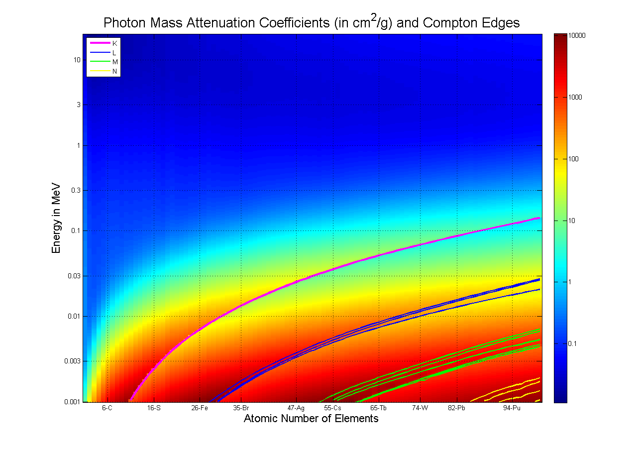
| תיאור | Photon Mass Attenuation Coefficient for photons in energy range from 1 keV to 20 MeV for Elements Z = 1 to 100. Based on [1]. Also shown are locations of Compton edges. |
| תאריך יצירה | |
| מקור | נוצר על־ידי מעלה היצירה |
| יוצר | Jarekt |
| גרסאות אחרות | SVG version of the same image can be found at Image:Photon Mass Attenuation Coefficients.svg, however it is larger and does not seem to render correctly |
. MATLAB עם נוצרה ה PNG תמונת מפת סיביות
The image was generated using the following MATLAB code, with help of external library PhotonAtenuattion2:
figure
Z = 1:100;  % elements with Z in 1-100 range - number of columns
nr = 500;   % number of rows to use in the plot
E = logspace(log10(0.001), log10(20), 500);  % define energy grid
[mac, CEdge] = PhotonAttenuationQ(Z, E);
colormap(jet(128)) % use hi-res color palette
imagesc(log10(mac));
grid on;
axis xy; % put small numbers on y axis on the bottom
title('Photon Mass Attenuation Coefficients (in cm^2/g) and Compton Edges');
xlabel('Atomic Number of Elements');
ylabel('Energy in MeV');
% Add X-Axis
EPos = [6 16 26 35 47 55 65 74 82 94];   % define array to store label location
ELab = { '6-C','16-S','26-Fe','35-Br','47-Ag','55-Cs','65-Tb','74-W','82-Pb','94-Pu'}; %Define Energy labels for y-axis
set(gca,'XTick'     ,EPos);
set(gca,'XTickLabel',ELab);
% Add Y-Axis
ELab = [0.001 0.003 0.01 0.03 0.1 0.3 1 3 10]; %Define Energy labels for y-axis
EPos = size(ELab);   % define array to store label location
for i=1:length(ELab), [tmp EPos(i)]=min(abs(E-ELab(i))); end
set(gca,'YTick'     ,EPos);
set(gca,'YTickLabel',ELab);
% add Colorbar
cbar_axes = colorbar;
set(cbar_axes,'YTick'     ,     -1:4 ); % The image is a log10 of the MAC ...
set(cbar_axes,'YTickLabel',10.^(-1:4)); % ... so add proper labels
hold on
% Add Conpton Edges to the plot
ed = accumarray([CEdge(:,1),CEdge(:,2)],CEdge(:,3)); % get per element energies of 14 compton edges
ed = 500*(log(ed')-log(0.001))/(log(20)-log(0.001)); % convert energy to row numbers of the image
K=plot(ed(:,1)    ,'m','LineWidth',3); %Plot K Compton edge
L=plot(ed(:, 2: 4),'b','LineWidth',2); %Plot 3 L Compton edges
M=plot(ed(:, 5: 9),'g','LineWidth',2); %Plot 5 M Compton edges
N=plot(ed(:,10:14),'Y','LineWidth',2); %Plot first 5 N Compton edges
legend([K(1),L(1),M(1),N(1)], {'K','L','M','N'}, 'Location', 'NorthWest');
רישיון
אני, בעל זכויות היוצרים על היצירה הזאת, מפרסם אותה בזאת תחת הרישיונות הבאים:

|
מוענקת בכך הרשות להעתיק, להפיץ או לשנות את המסמך הזה, לפי תנאי הרישיון לשימוש חופשי במסמכים של גנו, גרסה 1.2 או כל גרסה מאוחרת יותר שתפורסם על־ידי המוסד לתוכנה חופשית; ללא פרקים קבועים, ללא טקסט עטיפה קדמית וללא טקסט עטיפה אחורית. עותק של הרישיון כלול בפרק שכותרתו הרישיון לשימוש חופשי במסמכים של גנו. |
הקובץ הזה מתפרסם לפי תנאי רישיונות קריאייטיב קומונז ייחוס-שיתוף זהה 3.0 לא מותאם, 2.5 כללי, 2.0 כללי ו־1.0 כללי.
- הנכם רשאים:
- לשתף – להעתיק, להפיץ ולהעביר את העבודה
- לערבב בין עבודות – להתאים את העבודה
- תחת התנאים הבאים:
- ייחוס – יש לתת ייחוס הולם, לתת קישור לרישיון, ולציין אם נעשו שינויים. אפשר לעשות את זה בכל צורה סבירה, אבל לא בשום צורה שמשתמע ממנה שמעניק הרישיון תומך בך או בשימוש שלך.
- שיתוף זהה – אם תיצרו רמיקס, תשנו, או תבנו על החומר, חובה עליכם להפיץ את התרומות שלך לפי תנאי רישיון זהה או תואם למקור.
הנכם מוזמנים לבחור את הרישיון הרצוי בעיניכם.
היסטוריית הקובץ
ניתן ללחוץ על תאריך/שעה כדי לראות את הקובץ כפי שנראה באותו זמן.
| תאריך/שעה | תמונה ממוזערת | ממדים | משתמש | הערה | |
|---|---|---|---|---|---|
| נוכחית | 04:36, 27 בספטמבר 2007 | | 908 × 1,280 (55 ק"ב) | Jarekt | {{Information |Description=Photon '''Mass Attenuation Coefficient''' for photons in energy range from 1 keV to 20 MeV for Elements Z = 1 to 100. Based on [http://physics.nist.gov/PhysRefData/XrayNoteB.html]. Also shown are locations of Compton edges. |Sou |
שימוש בקובץ
![]() אין בוויקיפדיה דפים המשתמשים בקובץ זה.
אין בוויקיפדיה דפים המשתמשים בקובץ זה.
שימוש גלובלי בקובץ
אתרי הוויקי השונים הבאים משתמשים בקובץ זה:
- שימוש באתר en.wikipedia.org
- שימוש באתר ja.wikipedia.org