
קובץ:Bloop locations.png
גודל התצוגה המקדימה הזאת: 600 × 600 פיקסלים. רזולוציות אחרות: 240 × 240 פיקסלים | 480 × 480 פיקסלים | 768 × 768 פיקסלים | 1,024 × 1,024 פיקסלים | 2,048 × 2,048 פיקסלים | 3,000 × 3,000 פיקסלים.
לקובץ המקורי (3,000 × 3,000 פיקסלים, גודל הקובץ: 7.74 מ"ב, סוג MIME: image/png)
| זהו קובץ שמקורו במיזם ויקישיתוף. תיאורו בדף תיאור הקובץ המקורי (בעברית) מוצג למטה. |
תקציר
| תיאור |
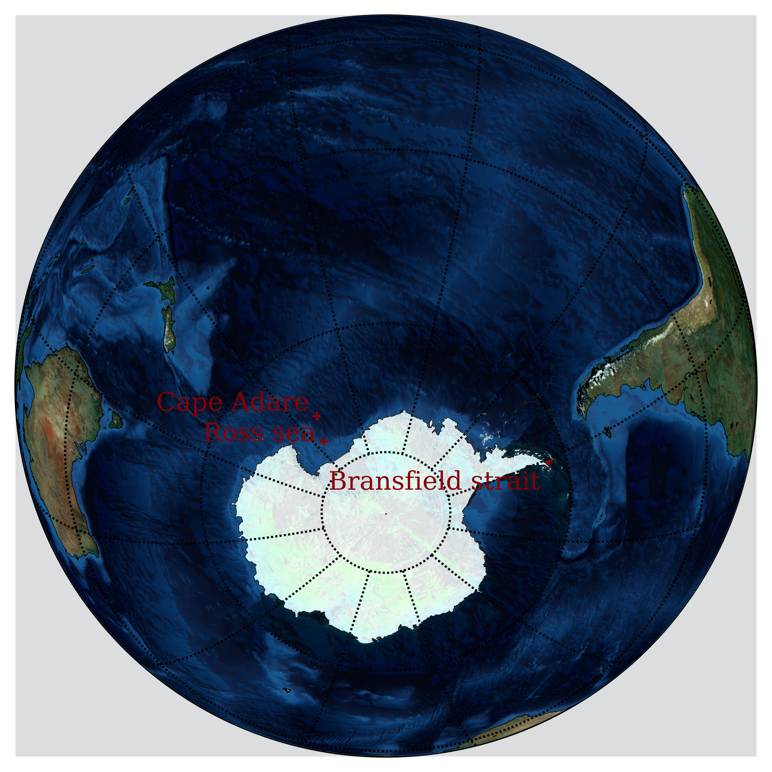
English: Possible locations of the Bloop, an ultra-low frequency and extremely powerful underwater sound detected by the U.S. National Oceanic and Atmospheric Administration (NOAA) in 1997. |
| תאריך יצירה | |
| מקור | נוצר על־ידי מעלה היצירה |
| יוצר | Nojhan |
| PNGהתפתחות | Python עם נוצרה ה PNG תמונת מפת סיביות |
Source code
This image has been generated by the following source code in Python:
Python code
| source code |
|---|
print "import modules...",
import sys
sys.stdout.flush()
import pickle
from mpl_toolkits.basemap import Basemap, shiftgrid, cm
import matplotlib
import matplotlib.pyplot as plt
import numpy as np
from netCDF4 import Dataset
print "ok"

# Lovecraft: 47:9'S 126:43'W
# lovecraft_lat = -47.9
# lovecraft_lon = -126.43

# August Derleth: 49:51'S 128:34'W
# derleth_lat = -49.51
# derleth_lon = -128.34

# Nemo point: 48:52.6'S 123:23.6'W
# nemo_lat = -48.526
# nemo_lon = -123.236

# The Bloop:
bransfield_strait_lat=-63
bransfield_strait_lon=-59
ross_sea_lat = -75
ross_sea_lon = -175
cape_adare_lat = -71.17
cape_adare_lon = -170.14

mid_lat = np.mean((bransfield_strait_lat,ross_sea_lat,cape_adare_lat))
mid_lon = np.mean((bransfield_strait_lon,ross_sea_lon,cape_adare_lon))


# Not necessary, because the default projection is ortho,
# but can be useful if you want another one.
def equi(m, centerlon, centerlat, radius, *args, **kwargs):
    """
    Drawing circles of a given radius around any point on earth, given the current projection.
    http://www.geophysique.be/2011/02/20/matplotlib-basemap-tutorial-09-drawing-circles/
    """
    glon1 = centerlon
    glat1 = centerlat
    X = []
    Y = []
    for azimuth in range(0, 360):
        glon2, glat2, baz = shoot(glon1, glat1, azimuth, radius)
        X.append(glon2)
        Y.append(glat2)
    X.append(X[0])
    Y.append(Y[0])

    #m.plot(X,Y,**kwargs) #Should work, but doesn't...
    X,Y = m(X,Y)
    plt.plot(X,Y,**kwargs)


def shoot(lon, lat, azimuth, maxdist=None):
    """Shooter Function
    Plotting great circles with Basemap, but knowing only the longitude,
    latitude, the azimuth and a distance. Only the origin point is known.
    Original javascript on http://williams.best.vwh.net/gccalc.htm
    Translated to python by Thomas Lecocq :
    http://www.geophysique.be/2011/02/19/matplotlib-basemap-tutorial-08-shooting-great-circles/
    """
    glat1 = lat * np.pi / 180.
    glon1 = lon * np.pi / 180.
    s = maxdist / 1.852
    faz = azimuth * np.pi / 180.

    EPS= 0.00000000005
    if ((np.abs(np.cos(glat1))<EPS) and not (np.abs(np.sin(faz))<EPS)):
        alert("Only N-S courses are meaningful, starting at a pole!")

    a=6378.13/1.852
    f=1/298.257223563
    r = 1 - f
    tu = r * np.tan(glat1)
    sf = np.sin(faz)
    cf = np.cos(faz)
    if (cf==0):
        b=0.
    else:
        b=2. * np.arctan2 (tu, cf)

    cu = 1. / np.sqrt(1 + tu * tu)
    su = tu * cu
    sa = cu * sf
    c2a = 1 - sa * sa
    x = 1. + np.sqrt(1. + c2a * (1. / (r * r) - 1.))
    x = (x - 2.) / x
    c = 1. - x
    c = (x * x / 4. + 1.) / c
    d = (0.375 * x * x - 1.) * x
    tu = s / (r * a * c)
    y = tu
    c = y + 1
    while (np.abs (y - c) > EPS):

        sy = np.sin(y)
        cy = np.cos(y)
        cz = np.cos(b + y)
        e = 2. * cz * cz - 1.
        c = y
        x = e * cy
        y = e + e - 1.
        y = (((sy * sy * 4. - 3.) * y * cz * d / 6. + x) *
              d / 4. - cz) * sy * d + tu

    b = cu * cy * cf - su * sy
    c = r * np.sqrt(sa * sa + b * b)
    d = su * cy + cu * sy * cf
    glat2 = (np.arctan2(d, c) + np.pi) % (2*np.pi) - np.pi
    c = cu * cy - su * sy * cf
    x = np.arctan2(sy * sf, c)
    c = ((-3. * c2a + 4.) * f + 4.) * c2a * f / 16.
    d = ((e * cy * c + cz) * sy * c + y) * sa
    glon2 = ((glon1 + x - (1. - c) * d * f + np.pi) % (2*np.pi)) - np.pi

    baz = (np.arctan2(sa, b) + np.pi) % (2 * np.pi)

    glon2 *= 180./np.pi
    glat2 *= 180./np.pi
    baz *= 180./np.pi

    return (glon2, glat2, baz)


print "read in etopo5 topography/bathymetry"
url = 'http://ferret.pmel.noaa.gov/thredds/dodsC/data/PMEL/etopo5.nc'
etopodata = Dataset(url)

print "get data"

def topopickle(etopodata,name):
    import sys
    print "\t"+name+"...",
    sys.stdout.flush()
    filename = "rlyeh_"+name+".pickle"
    try:
        with open(filename,"r") as fd:
            print "load...",
            var = pickle.load(fd)
    except IOError:
        print "copy...",
        var = etopodata.variables[name][:]
        with open(filename,"w") as fd:
            print "dump...",
            pickle.dump(var,fd)
    print "ok"
    return var

topoin = topopickle(etopodata,"ROSE")
lons   = topopickle(etopodata,"ETOPO05_X")
lats   = topopickle(etopodata,"ETOPO05_Y")
print "shift data so lons go from -180 to 180 instead of 20 to 380...",
sys.stdout.flush()
topoin,lons = shiftgrid(180.,topoin,lons,start=False)
print "ok"


# create the figure and axes instances.
fig = plt.figure()
ax = fig.add_axes([0.1,0.1,0.8,0.8])

print "setup basemap"
# set up orthographic m projection with
# perspective of satellite looking down at 50N, 100W.
# use low resolution coastlines.
m = Basemap(projection='ortho',lat_0=mid_lat,lon_0=mid_lon,resolution='l')
m.bluemarble()

# Generic Mapping Tools colormaps:
# GMT_drywet, GMT_gebco, GMT_globe, GMT_haxby GMT_no_green, GMT_ocean, GMT_polar,
# GMT_red2green, GMT_relief, GMT_split, GMT_wysiwyg

print "transform to nx x ny regularly spaced native projection grid"
# step=5000.
step=10000.
nx = int((m.xmax-m.xmin)/step)+1; ny = int((m.ymax-m.ymin)/step)+1
topodat = m.transform_scalar(topoin,lons,lats,nx,ny)

print "plot topography/bathymetry as shadows"
from matplotlib.colors import LightSource
ls = LightSource(azdeg = 45, altdeg = 220, hsv_min_val=0.0, hsv_max_val=1.0,
        hsv_min_sat=0.0, hsv_max_sat=1.0)
# convert data to rgb array including shading from light source.
# (must specify color m)
rgb = ls.shade(topodat, cm.GMT_ocean)
im = m.imshow(rgb, alpha=0.15)

print "draw coastlines, country boundaries, fill continents"
m.drawcoastlines(linewidth=0.25)
# draw the edge of the map projection region
m.drawmapboundary(fill_color='white')
# draw lat/lon grid lines every 30 degrees.
m.drawmeridians(np.arange(  0,360,30), color="black" )
m.drawparallels(np.arange(-90,90 ,30), color="black" )

print "draw points"
psize=5
font = {'family' : 'serif',
        'weight' : 'normal',
        'size'   : 12}
matplotlib.rc('font', **font)

# x,y = m( lovecraft_lon, lovecraft_lat )
# m.scatter(x,y,psize,marker='o', color='white')
# plt.text(x+50000,y+50000+50000, "Lovecraft", color='white')
#
# x,y = m( derleth_lon, derleth_lat )
# m.scatter(x,y,psize,marker='o',color='white')
# plt.text(x+50000-120000,y+50000, "Derleth", color='white', horizontalalignment="right")

# x,y = m( nemo_lon, nemo_lat )
# m.scatter(x,y,psize*3,marker='+',color='#555555')
# plt.text(x+50000+50000,y+50000-80000, "Nemo", color="#555555", verticalalignment="top")
#
# equi(m, nemo_lon, nemo_lat, radius=2688, color="#555555" )

pcolor="darkred"
offset=150000

x,y = m( bransfield_strait_lon, bransfield_strait_lat )
m.scatter(x,y,psize*3,marker='+',color=pcolor)
plt.text(x-offset,y-offset, "Bransfield strait", color=pcolor,
        horizontalalignment="right", verticalalignment="top")

x,y = m( ross_sea_lon, ross_sea_lat )
m.scatter(x,y,psize*3,marker='+',color=pcolor)
plt.text(x-offset,y, "Ross sea", color=pcolor,
        horizontalalignment="right", verticalalignment="bottom")

x,y = m( cape_adare_lon, cape_adare_lat )
m.scatter(x,y,psize*3,marker='+',color=pcolor)
plt.text(x-offset,y, "Cape Adare", color=pcolor,
        horizontalalignment="right", verticalalignment="bottom")

plt.savefig("Bloop_locations.png", dpi=600, bbox_inches='tight')
# plt.show()
|
רישיון
אני, בעל זכויות היוצרים על עבודה זו, מפרסם בזאת את העבודה תחת הרישיון הבא:
הקובץ הזה מתפרסם לפי תנאי רישיון קריאייטיב קומונז ייחוס-שיתוף זהה 3.0 לא מותאם.
- הנכם רשאים:
- לשתף – להעתיק, להפיץ ולהעביר את העבודה
- לערבב בין עבודות – להתאים את העבודה
- תחת התנאים הבאים:
- ייחוס – יש לתת ייחוס הולם, לתת קישור לרישיון, ולציין אם נעשו שינויים. אפשר לעשות את זה בכל צורה סבירה, אבל לא בשום צורה שמשתמע ממנה שמעניק הרישיון תומך בך או בשימוש שלך.
- שיתוף זהה – אם תיצרו רמיקס, תשנו, או תבנו על החומר, חובה עליכם להפיץ את התרומות שלך לפי תנאי רישיון זהה או תואם למקור.
היסטוריית הקובץ
ניתן ללחוץ על תאריך/שעה כדי לראות את הקובץ כפי שנראה באותו זמן.
| תאריך/שעה | תמונה ממוזערת | ממדים | משתמש | הערה | |
|---|---|---|---|---|---|
| נוכחית | 00:46, 13 בפברואר 2013 | | 3,000 × 3,000 (7.74 מ"ב) | Nojhan | User created page with UploadWizard |
שימוש בקובץ
![]() אין בוויקיפדיה דפים המשתמשים בקובץ זה.
אין בוויקיפדיה דפים המשתמשים בקובץ זה.
שימוש גלובלי בקובץ
אתרי הוויקי השונים הבאים משתמשים בקובץ זה: